10 Google Sheets Formulas Every SEO Should Know

Google Sheets is free, cloud-based, and does almost everything Excel can do. But most SEOs only scratch the surface. They sort columns, maybe highlight duplicates, and stop there.

That leaves hours of manual work on the table.

The formulas in this guide will help you extract domains from messy URL lists, merge data from multiple sources, scrape metadata without leaving your spreadsheet, categorize thousands of keywords in seconds, and query large data sets with precision. Each formula includes the syntax, a practical SEO example, and a few bonus use cases so you can adapt it to your own workflow.

And because SEO is evolving to include AI search as an additional organic channel, we’ll also show you how to use these same formulas to analyze AI search data. Things like which AI engines mention your brand, which landing pages receive AI-referred traffic, and where competitors outrank you in AI answers.

In this article, you’ll learn 10 Google Sheets formulas that handle the most common (and most tedious) SEO tasks. You’ll see the exact syntax, real examples with SEO data, and step-by-step use cases you can copy into your own spreadsheets. You’ll also learn how to apply these same formulas to a newer challenge: analyzing your brand’s visibility across AI search engines like ChatGPT, Perplexity, and Gemini.

Three formulas you’ll use in almost every spreadsheet

Before we get into the more advanced stuff, you need three foundational formulas. These show up in nearly every SEO spreadsheet, and the rest of this guide builds on them.

IF

IF checks whether a condition is true or false, then returns one value for true and another for false.

Syntax: =IF(condition, value_if_true, value_if_false)

Here’s a practical example. Say you exported a list of keywords and their monthly search volumes from a keyword research tool. You want to flag every keyword with 1,000+ monthly searches as “High Priority” and everything else as “Low Priority.”

The formula:

=IF(B2>=1000, "High Priority", "Low Priority")

This works for a single cell. But what happens when your search volume column has a blank cell or a text value like “N/A”? The formula breaks. That’s where IFERROR comes in.

IFERROR

IFERROR wraps around any formula and returns a fallback value when the formula produces an error. Instead of seeing #VALUE! or #REF! scattered across your sheet, you get a clean result.

Syntax: =IFERROR(original_formula, value_if_error)

Let’s fix the IF formula from above so it handles bad data gracefully:

=IFERROR(IF(B2>=1000, "High Priority", "Low Priority"), "No Data")

Now, any row with missing or non-numeric search volume data will show “No Data” instead of an error.

ARRAYFORMULA

If you’ve ever dragged a formula down across hundreds or thousands of rows, you already know why ARRAYFORMULA exists. It lets you write one formula in one cell and apply it to an entire column at once.

Syntax: =ARRAYFORMULA(formula_using_ranges)

Here’s how to combine all three foundational formulas into a single cell that processes your entire keyword list:

=ARRAYFORMULA(IFERROR(IF(B2:B>=1000, "High Priority", "Low Priority"), "No Data"))

Put this in cell C2, and it fills down automatically for every row that has data in column B. No dragging. No copying. One formula, unlimited rows.

These three formulas are the backbone of every workflow in this guide. Most of the formulas below will be wrapped in IFERROR and ARRAYFORMULA, so get comfortable with them now.

1. VLOOKUP: Merge data sets from multiple sources

VLOOKUP searches for a value in the first column of a range and returns a corresponding value from another column. It’s the formula you’ll reach for every time you need to combine data from two different sources into one sheet.

Syntax: =VLOOKUP(search_key, range, column_index, [is_sorted])

Set is_sorted to FALSE for exact matches (which is almost always what you want in SEO work).

SEO use case: Merge keyword data with ranking data

You exported a keyword list with search volumes from one tool, and a separate ranking report from Google Search Console. Both sheets share a common column (the keyword). You want to pull the ranking position into your keyword sheet.

Step 1: Put your keyword list with search volumes in Sheet1.

Step 2: Put your Search Console ranking data in Sheet2. Make sure the keyword column is the first column.

Step 3: In Sheet1, add a new column for “Current Position” and enter:

=IFERROR(VLOOKUP(A2, Sheet2!A:C, 3, FALSE), "Not Ranking")

This searches for the keyword in A2 across Sheet2, and returns the value from the third column (position). If the keyword isn’t found, it returns “Not Ranking.”

Step 4: Wrap it in an ARRAYFORMULA to fill the entire column:

=ARRAYFORMULA(IFERROR(VLOOKUP(A2:A, Sheet2!A:C, 3, FALSE), "Not Ranking"))

More VLOOKUP use cases for SEO

You can use the same pattern to merge backlink data with domain authority scores, pull contact information from a master outreach database alongside a list of link prospects, or match URLs from a crawl report with their corresponding organic traffic numbers from analytics.

How to merge AI search data with your SEO data

If you’re tracking how your brand appears in AI search engines, the data starts in a different place but the formula is identical.

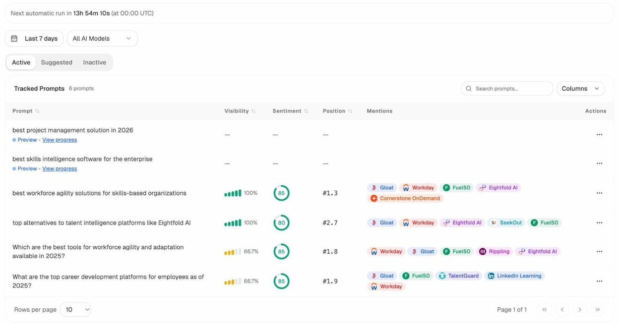
For example, Analyze AI tracks which prompts mention your brand across ChatGPT, Perplexity, Gemini, and other AI engines. You can export this prompt-level data and use VLOOKUP to merge it with your traditional keyword tracking data.

Say you have a sheet of target keywords with their Google rankings, and a separate export from Analyze AI’s Prompt Tracking showing which AI prompts mention your brand, your visibility score, and your position.

The VLOOKUP formula to pull AI visibility into your keyword sheet:

=IFERROR(VLOOKUP(A2, 'AI Prompt Data'!A:D, 3, FALSE), "Not Tracked")

Now you have one spreadsheet showing both your Google ranking and your AI search visibility for each keyword. That’s a powerful way to spot gaps. A keyword where you rank #3 on Google but don’t appear in any AI answers is an opportunity. A keyword where AI engines recommend you but Google doesn’t rank you yet tells you something different about your content’s authority.

Use Analyze AI’s free Keyword Rank Checker to quickly pull your Google positions, then merge that with your AI visibility data using VLOOKUP.

2. REGEXEXTRACT: Pull specific data from messy strings

REGEXEXTRACT uses regular expressions to extract a piece of text from a longer string. If you’ve ever needed to pull the domain name from a URL, the protocol from a link, or the category slug from a blog post URL, this is the formula.

Syntax: =REGEXEXTRACT(text, regular_expression)

SEO use case: Extract root domains from a list of URLs

You ran a backlink audit and now have a list of 500 referring page URLs. You need the root domains so you can check their authority, spot patterns, and remove duplicates.

The formula:

=REGEXEXTRACT(A2, "^(?:https?://)?(?:www\.)?([^:/]+)")

This strips out the protocol (http/https), removes “www.” if present, and returns just the domain name.

Wrap it for the full column:

=ARRAYFORMULA(IFERROR(REGEXEXTRACT(A2:A, "^(?:https?://)?(?:www\.)?([^:/]+)"), ""))

More REGEXEXTRACT patterns for SEO

Here are a few regex patterns you’ll use regularly:

If you’re not familiar with regex, that’s normal. Most SEOs aren’t. Use a tool like Regexr.com to test patterns, or search for the exact pattern you need. Chances are, someone has already written it.

Bonus: Extract AI engine names from referrer data

If you’re analyzing AI traffic in Google Analytics or from an AI traffic analytics export, you’ll often have referrer URLs like chatgpt.com, claude.ai, or gemini.google.com. You can use REGEXEXTRACT to categorize these:

=IF(REGEXMATCH(A2, "chatgpt"), "ChatGPT",
IF(REGEXMATCH(A2, "claude"), "Claude",
IF(REGEXMATCH(A2, "gemini"), "Gemini",
IF(REGEXMATCH(A2, "perplexity"), "Perplexity",
IF(REGEXMATCH(A2, "copilot"), "Copilot", "Other")))))

This takes your raw referrer data and tags each row with the AI engine name, making it easy to pivot and analyze.

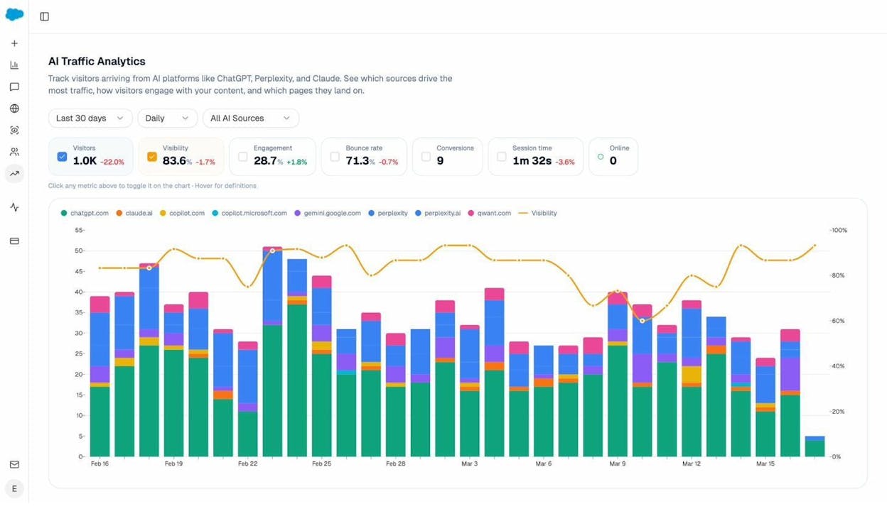
Analyze AI does this categorization automatically when you connect GA4, but this formula is useful when you want to run your own analysis or combine AI referrer data with other metrics in a custom sheet.

3. SPLIT: Break strings into multiple columns

SPLIT takes a text string and divides it into separate cells using a delimiter you specify. Anywhere the delimiter appears in the string, SPLIT makes a cut.

Syntax: =SPLIT(text, delimiter)

SEO use case: Split full names for outreach personalization

You have a list of blog authors or webmasters you want to contact for link building. The names are in “First Last” format, but your email template needs the first name in one field and last name in another.

=SPLIT(A2, " ")

This splits “John Smith” into two cells: “John” in column B and “Smith” in column C.

For the full column:

=ARRAYFORMULA(IFERROR(SPLIT(A2:A, " "), ""))

SEO use case: Break URLs into components

You can also use SPLIT to break URLs into analyzable parts. Split a URL by “/” and you get the protocol, domain, and each folder in the path as separate columns:

=SPLIT(A2, "/")

This turns https://example.com/blog/seo-guide into separate cells containing https:, (blank), example.com, blog, and seo-guide.

More SPLIT use cases

You can split comma-separated tag lists into individual columns, break domain names at the dot to separate the name from the extension (e.g., “example” and “com”), or split keyword phrases by space to count word count per keyword.

4. IMPORTXML: Scrape data from any website

IMPORTXML pulls data from web pages directly into Google Sheets using XPath queries. No code required. No browser extensions. Just a formula.

Syntax: =IMPORTXML(url, xpath_query)

SEO use case: Scrape title tags from a list of URLs

You’re running a content audit and need to check the title tags for 50 pages. Instead of opening each page and viewing the source code, pull them all into a spreadsheet.

Put your URLs in column A. In column B, enter:

=IMPORTXML(A2, "//title")

Google Sheets will fetch the page and return the content of the <title> tag.

Essential XPath queries for SEO

Here are the XPath queries you’ll use most:

How to find the XPath for any element

If you need to scrape something not listed above, open the page in Chrome, right-click the element, select “Inspect,” then right-click the highlighted HTML and choose Copy > Copy XPath.

Limitations to know

IMPORTXML has a few quirks. It doesn’t work with ARRAYFORMULA, so you’ll need to drag it down manually. Google Sheets also limits the number of IMPORTXML calls per sheet (usually around 50), and it can be slow on pages with heavy JavaScript rendering.

For larger-scale scraping jobs, a dedicated crawler like Screaming Frog is a better fit. But for quick checks on a handful of URLs, IMPORTXML is hard to beat.

Bonus: Check if your pages have structured data

You can use IMPORTXML to detect whether a page has JSON-LD structured data:

=IFERROR(IMPORTXML(A2, "//script[@type='application/ld+json']"), "No Schema Found")

This returns the raw JSON-LD content if it exists, or “No Schema Found” if the page lacks structured data. Use this during a technical SEO audit to flag pages that need schema markup.

5. SEARCH and FIND: Locate values inside strings

SEARCH checks whether a specific value exists within a text string and returns the position where it’s found. FIND does the same thing but is case-sensitive. For most SEO work, SEARCH is the one you want.

Syntax: =SEARCH(search_query, text_to_search)

On its own, SEARCH returns a number (the character position). That’s not very useful. The power comes when you combine it with IF to create tags and categories.

SEO use case: Tag blog posts in a URL list

You exported the top 500 pages from your site. You want to tag every URL that contains “/blog/” as a blog post.

=IF(IFERROR(SEARCH("/blog/", A2), 0), "Blog Post", "Other Page")

This checks if “/blog/” appears anywhere in the URL. If it does, the cell shows “Blog Post.” If not, “Other Page.”

SEO use case: Categorize keywords by intent

You have a keyword list and want to segment it by search intent. You can use nested SEARCH formulas to flag commercial keywords (containing words like “best,” “top,” “review,” “vs,” “alternative”):

=IF(IFERROR(SEARCH("best", A2), 0) + IFERROR(SEARCH("top", A2), 0) + IFERROR(SEARCH("review", A2), 0) + IFERROR(SEARCH("vs", A2), 0) + IFERROR(SEARCH("alternative", A2), 0) > 0, "Commercial", "Informational")

This is a rough pass, not a perfect classifier. But it saves significant time when you’re working through a large keyword list and need to prioritize keywords by type.

More SEARCH patterns for SEO

Tagging AI search prompts by topic

If you export prompt data from Analyze AI’s Prompt Discovery, you can use SEARCH to group prompts by topic cluster. For example, if you’re a CRM company, you might tag prompts containing “enterprise” separately from those containing “small business”:

=IF(IFERROR(SEARCH("enterprise", A2), 0), "Enterprise",
IF(IFERROR(SEARCH("small business", A2), 0), "SMB",
IF(IFERROR(SEARCH("startup", A2), 0), "Startup", "General")))

This helps you quickly see which customer segments AI engines associate with your brand and where there are competitive gaps.

6. IMPORTRANGE: Pull data from other spreadsheets

IMPORTRANGE imports data from any Google Sheet you have access to. This is essential when you maintain separate spreadsheets for different projects, clients, or data sources and need to consolidate without copy-pasting.

Syntax: =IMPORTRANGE(spreadsheet_url, range_string)

SEO use case: Build a master dashboard from multiple client sheets

You manage SEO for five clients, each with their own reporting spreadsheet. You want a single master dashboard that shows the latest metrics for all clients.

Step 1: Get the spreadsheet URL (or just the key) for each client sheet.

Step 2: In your master dashboard, pull in the data:

=IMPORTRANGE("https://docs.google.com/spreadsheets/d/SPREADSHEET_KEY", "'Monthly Report'!A2:D10")

Step 3: The first time you use IMPORTRANGE with a new spreadsheet, Google Sheets will ask you to allow access. Click “Allow access” and the data will populate.

SEO use case: Create a dropdown from a master list

You can combine IMPORTRANGE with Data Validation to create dynamic dropdowns that stay in sync with a master list.

For example, if you maintain a master spreadsheet of all your link building prospects, you can create a dropdown in your outreach tracking sheet that automatically updates when you add new prospects to the master list.

Step 1: In your outreach sheet, create a hidden tab and use IMPORTRANGE to pull in the prospect list from the master sheet.

Step 2: Set up a Data Validation rule on your tracking column that references the imported range.

Now when your team adds a prospect to the master list, it automatically appears in the dropdown on the outreach sheet. No manual updates needed.

Cross-referencing SEO data with AI visibility data

IMPORTRANGE is particularly useful when your traditional SEO data lives in one spreadsheet (maybe fed by Google Search Console or a rank tracking tool) and your AI search data lives in another (maybe exported from Analyze AI).

Pull both into a single analysis sheet:

=IMPORTRANGE("SEO_DATA_SHEET_URL", "'Rankings'!A:E")

=IMPORTRANGE("AI_VISIBILITY_SHEET_URL", "'Prompt Data'!A:F")

Then use VLOOKUP (covered in section 1) to match keywords across both data sets. This gives you a single view of where you stand in both traditional search and AI search for every target keyword.

7. QUERY: Run SQL-style queries on your data

QUERY is the most powerful formula in Google Sheets. It lets you filter, sort, aggregate, and manipulate data using a syntax similar to SQL. If you only learn one formula on this list, make it this one.

Syntax: =QUERY(data_range, query_string, [headers])

SEO use case: Filter a backlink report to find high-quality prospects

You exported a backlink report and have columns for referring domain, DR (Domain Rating), link type (dofollow/nofollow), anchor text, and target URL. You want to pull only dofollow links from domains with a DR above 40.

=QUERY('Backlink Data'!A:F, "SELECT A, B, D WHERE C > 40 AND E = 'Dofollow'", 1)

This returns only the rows that match both conditions, showing just the columns you specified. No manual filtering. No deleting rows. One formula.

SEO use case: Group keywords by search volume range

You want to see how many keywords fall into each search volume bracket. QUERY can aggregate this:

=QUERY(A:B, "SELECT A, B WHERE B >= 1000 ORDER BY B DESC", 1)

This gives you all keywords with 1,000+ monthly search volume, sorted from highest to lowest.

More QUERY patterns for SEO

How to use QUERY with AI search data

If you export data from Analyze AI’s Competitor Intelligence or Citation Analytics, QUERY becomes a fast way to slice it.

For example, say you exported a list of every prompt where your competitors appear but you don’t. You want to filter that list to show only prompts with a commercial intent:

=QUERY('Competitor Prompts'!A:E, "SELECT A, B, C WHERE D = 'Not Visible' AND (A CONTAINS 'best' OR A CONTAINS 'top' OR A CONTAINS 'alternative')", 1)

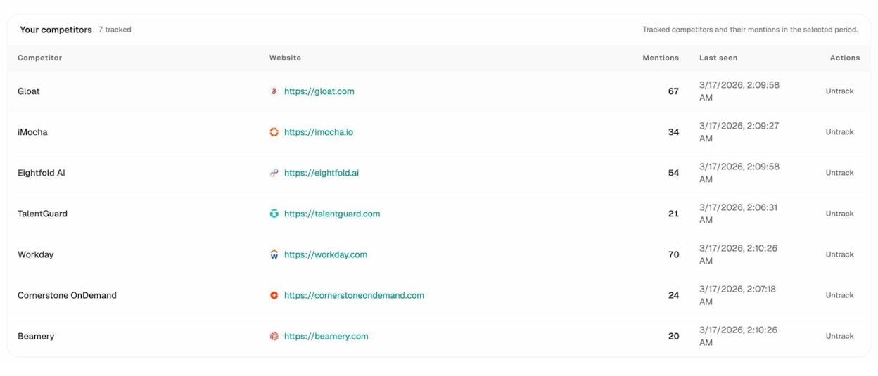
This gives you a focused list of high-value prompts where competitors are winning and you’re absent. Feed these into Analyze AI’s Prompt Tracking to start monitoring them automatically, and use the insights to guide what content to create or optimize next.

8. CONCATENATE and TEXTJOIN: Combine data into single cells

CONCATENATE joins text strings together. TEXTJOIN does the same thing but adds a delimiter between each value and can skip empty cells. For most use cases, TEXTJOIN is the better choice.

Syntax:

=CONCATENATE(string1, string2, ...)
=TEXTJOIN(delimiter, ignore_empty, string1, string2, ...)

SEO use case: Build URLs from components

You’re creating a list of competitor pages to analyze. You have domains in one column and URL slugs in another. You need full URLs:

=CONCATENATE("https://", A2, "/", B2)

This turns “example.com” and “blog/seo-guide” into “https://example.com/blog/seo-guide”.

SEO use case: Create bulk title tag suggestions

You’re optimizing title tags for a batch of product pages. You have the product name, category, and brand name in separate columns. TEXTJOIN builds the title tag:

=TEXTJOIN(" | ", TRUE, A2, B2, "YourBrand")

This produces something like “Running Shoes | Athletic Footwear | YourBrand.”

SEO use case: Generate keyword variations at scale

Combine seed keywords with modifiers to build a list of long-tail variations:

=TEXTJOIN(CHAR(10), TRUE,
  CONCATENATE("best ", A2),
  CONCATENATE(A2, " for beginners"),
  CONCATENATE("how to choose ", A2),
  CONCATENATE(A2, " vs ", B2))

This generates four keyword variations per row. Use this to quickly build keyword lists that you can validate with Analyze AI’s free Keyword Generator or Keyword Difficulty Checker.

9. COUNTIF and COUNTIFS: Count what matters

COUNTIF counts how many cells in a range meet a single condition. COUNTIFS does the same but allows multiple conditions. These are essential for building summaries and finding patterns in large data sets.

Syntax:

=COUNTIF(range, condition)
=COUNTIFS(range1, condition1, range2, condition2, ...)

SEO use case: Count keyword distribution by intent

You categorized your keywords using the SEARCH formula from section 5. Now you want a summary showing how many keywords fall into each category:

=COUNTIF(C:C, "Commercial")
=COUNTIF(C:C, "Informational")

SEO use case: Find duplicate URLs in a crawl report

Want to quickly check if any URLs appear more than once in your data?

=COUNTIF(A:A, A2)

Any cell showing a number greater than 1 indicates a duplicate. Use Conditional Formatting to highlight these cells automatically.

If you’re dealing with broken links, duplicate content, or redirect chains, COUNTIF helps you quantify the problem before you start fixing it.

SEO use case: Count pages ranking in different position brackets

You want to know how many keywords rank in positions 1-3, 4-10, 11-20, and 20+:

=COUNTIFS(B:B, ">=1", B:B, "<=3")
=COUNTIFS(B:B, ">=4", B:B, "<=10")
=COUNTIFS(B:B, ">=11", B:B, "<=20")
=COUNTIF(B:B, ">20")

This gives you a distribution that shows where your SEO efforts are paying off and where pages need more work.

Counting AI search visibility gaps

If you’ve exported prompt data from Analyze AI, you can use COUNTIFS to count how many prompts you’re visible for versus how many you’re missing:

=COUNTIF(D:D, ">0")    // Prompts where you're visible
=COUNTIF(D:D, "0")      // Prompts where you're absent

This quick count tells you the scale of your AI visibility gap. From there, you can use Analyze AI’s Improve tools to figure out what content to create or optimize to close that gap, whether that’s for traditional search engines or AI search.

10. UNIQUE and FILTER: Clean and slice data instantly

UNIQUE removes duplicate values from a range. FILTER returns only the rows that meet your specified conditions. Together, they’re a fast alternative to manually sorting and deleting rows.

Syntax:

=UNIQUE(range)
=FILTER(range, condition1, [condition2, ...])

SEO use case: Deduplicate a list of referring domains

You exported backlinks from multiple sources and merged them. Now you have duplicate domains. UNIQUE cleans the list in one step:

=UNIQUE(A2:A)

SEO use case: Filter pages with declining traffic

You have a content performance sheet with URLs, last month’s traffic, and this month’s traffic. You want to see only the pages where traffic dropped:

=FILTER(A2:C, C2:C < B2:B)

This returns only the rows where this month’s traffic (column C) is lower than last month’s (column B). It’s the fastest way to build a list of pages that need a content refresh.

Bonus: Combine UNIQUE and FILTER

Find all unique domains that link to you with dofollow links:

=UNIQUE(FILTER(A2:A, B2:B = "Dofollow"))

This filters to only dofollow rows, then removes duplicates from the domain column. You get a clean list of unique referring domains with dofollow links, which is one of the most important metrics in any link building campaign.

Filtering AI citation sources

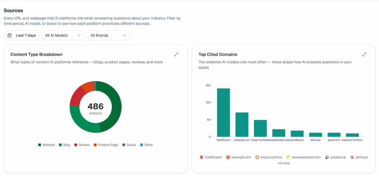
If you’re analyzing which sources AI engines cite in your industry (something Analyze AI’s Citation Analytics tracks automatically), you can export the data and use FILTER to find patterns:

=FILTER(A2:D, B2:B >= 5, C2:C = "Blog")

This shows only blog-type sources that have been cited five or more times. These are the sources AI engines trust in your space. If your own blog isn’t on that list, you know exactly what kind of content to create.

Putting it all together: Build an SEO + AI search analysis sheet

The formulas above are powerful on their own. They become even more useful when combined into a single analysis workflow.

Here’s a practical example of how you might combine them.

Step 1: Export your keyword rankings from Google Search Console or a rank tracker. Paste them into a sheet called “SEO Data.”

Step 2: Export your AI visibility data from Analyze AI. Paste it into a sheet called “AI Data.”

Step 3: In a new sheet called “Combined Analysis,” use VLOOKUP to merge both data sets by keyword:

=VLOOKUP(A2, 'SEO Data'!A:D, 3, FALSE)   // Pull Google position
=VLOOKUP(A2, 'AI Data'!A:E, 4, FALSE)      // Pull AI visibility score

Step 4: Use IF to flag opportunities:

=IF(AND(B2<=10, C2="Not Visible"), "AI Gap: Strong in Google, Weak in AI",
IF(AND(B2>20, C2>50), "SEO Gap: Strong in AI, Weak in Google",
IF(AND(B2<=10, C2>50), "Strong in Both", "Needs Work in Both")))

Step 5: Use QUERY to pull out just the most actionable items:

=QUERY('Combined Analysis'!A:D, "SELECT A, B, C, D WHERE D = 'AI Gap: Strong in Google, Weak in AI' ORDER BY B ASC", 1)

This gives you a prioritized list of keywords where you’re ranking well on Google but invisible to AI search engines. These are your lowest-hanging fruit for AI visibility, because the content already exists and ranks. It likely just needs optimization so AI models pick it up too.

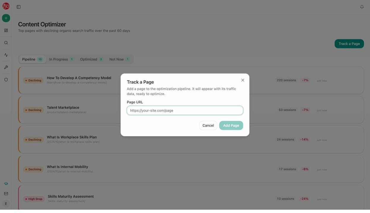
You can feed these URLs directly into Analyze AI’s Content Optimizer, which fetches your page, scores it, and gives you specific recommendations for what to change.

For keywords where you’re strong in AI but weak in Google, the insight is different. Your content has the depth and structure that AI models value, but it may need better on-page SEO, more backlinks, or improved technical performance to rank in traditional search.

Either way, the combined spreadsheet gives you a complete picture that neither data source provides alone.

Final thoughts

Google Sheets is one of the most underrated tools in an SEO’s stack. With these 10 formulas, you can process thousands of keywords in seconds, merge data from any source, scrape live pages without writing code, and build analysis workflows that would take hours to do manually.

And as AI search becomes an additional organic channel alongside traditional SEO, these same formulas work just as well on AI visibility data. The data is different, but the analysis patterns are the same. VLOOKUP still merges two data sets. QUERY still filters to the rows that matter. COUNTIF still quantifies the gap.

If you’re not tracking both channels yet, the Analyze AI free SERP Checker and AI Search Explorer are good places to start. Use them to see where you stand. Then open a spreadsheet, apply the formulas from this guide, and build your action plan.

The best SEOs don’t do more work. They build better systems. Google Sheets is where most of those systems start.